Getting Oris up and running

First of all, let's learn how to get Oris up and running.

Once you have Oris downloaded (link), head to the download folder and unzip the Oris archive you just downloaded.

Then, you can open the folder created and run Oris by simply running either run.bat, if you are on Windows, or run.sh, if you are on Linux or Mac.

Simple network creation

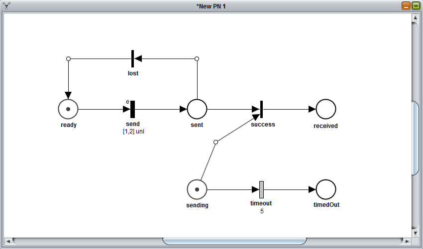
Now that we have Oris working and running we can start learning how to create our very first Petri Net with Oris following a simple example. The example Petri Net we're going to build will model a simple transmission with timeout on a lossy channel.

New network creation

The very first step is to create a new empty net by clicking the button from the toolbar. Alternatively, you can click File → New, from the menu, or use the shortcut Ctrl + N.

Adding places

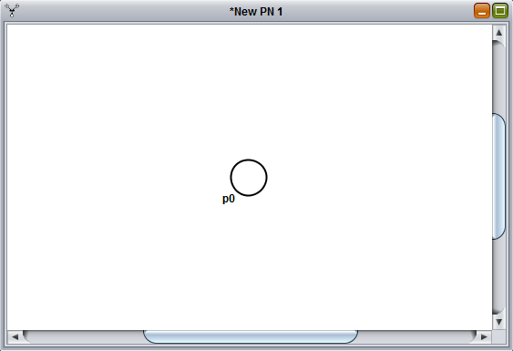
Let's start by adding a new place: to add a new place just click on the button and then on a random position on the canvas. You can see a new place will spawn, as shown below:

If we now double click on the place we just created, we can specify its name and the number of tokens in that place in the initial marking. Let's call it ready and give it one token, as shown below:

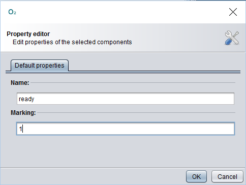
Now let's click OK to make the changes permanent.

Protip: If you select the button you'll enter in "selection mode" and be able, for example, to drag the place's name for a better readability.

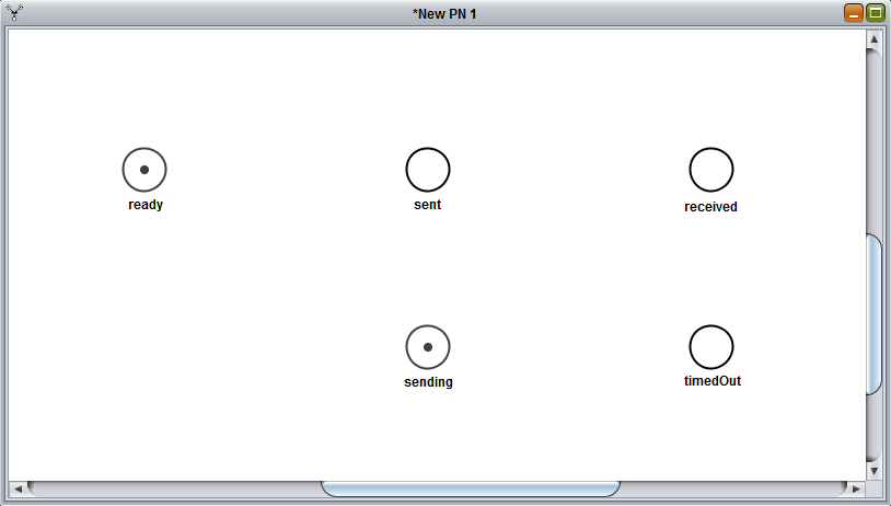
With the same method we've just seen, let's add four more places: sent, received and timedOut, with zero tokens, and sending, with one. For more clarity, the relative position of the places should be as shown below:

Adding transitions

Now that we have all the places we need set, let's add some transition.

The first transition we're gonna add will be a uniformely distributed transition, also called UNI: to create our new UNI transition let's select the button and click between the places ready and sent. Then, let's double click on the newly created transition to customize it's parameters as follows:

With these parameters we're basically telling the send transition to have a uniform probability distribution between 1 and 2 and to be able to fire only if the place timedOut has no marking (i.e. we want to send a message only if we've not yet timed out). Finally, selecting the , we can create an arc between a place and a transition (or viceversa) by dragging the arc from the starting element to the destination element: in this case let's create an arc from ready to send and another one from send to sent.

The result should be as follows:

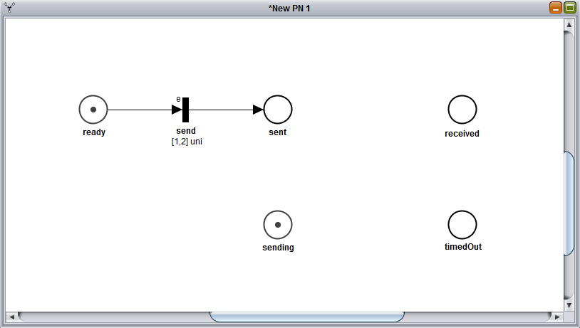
If you're wondering what does that little e on top of the transition means, it stands for enabling function, in this case it refers to the condition timedOut==0 we included in the transition.

Let's add three more transitions now.

The first will be a deterministiclally distributed transition (also called DET, added with the button). Let's call this one timeout and give it a value (Stochastic properties tab) of 5. This transition should be place between sending and timedOut, with an arc from sending to timeout and another one from timeout to timedOut.

Then, we want to add an immediate transition (a.k.a. IMM, button) just above the send transition. We'll call this one lost and will have an incoming arc from sent and an outgoing one towards ready.

Finally, we need a last IMM transition, between sent and received. This last transition, to be called success, should have two incoming arcs, one from sent and one from sending, and an outgoing one, towards received.

If done properly, the final result should be as follows:

Saving the PN

The Petri Net is now completed and ready to be used for various analyses.

Remember to save the Petri Net before closing, by clicking the button, if you want to reuse the net later. This process will generate a file in XPN format that contains the Petri Net description.

Some example STPNs

You can download and open the following example Stochastic Time Petri Nets (STPNs) in Oris (.xpn files) to experiment a bit around and learn how to do different kinds of analysis.

Regenerative transient analysis

One of the most useful analysis that can be conducted on a Petri Net is the regenerative transient analysis. This section, in particular, will cover a specific method of this kind of analysis: the regenerative transient analysis with stochastic state classes.

The transient analysis is the analysis of the probabilities of being in a certain state at a certain moment in time, given that the process started from another given state. This analysis generates a matrix, with time as the first dimension and the possible arrival states, starting from the initial marking, as second dimension.

Regenerative transient analysis indicates the transient analysis done on a generic Markov Regenerative Process (MPR). An MRP is a sthocastic process that, sooner or later, will certainly reach a regeneration (i.e. a moment in time where the past history of the process adds no information to the future probabilities).

Starting a new analysis

In this section we'll analyze the "Trasmission with Timeout" model we build in the previous section. If you don't have the model open in Oris (or you didn't save it) you can download it from the examples (link) and open it again.

Once we have the model back up on the main pane, we can start a new regenerative transient analysis by clicking the button. We'll notice a new panel, like the one below, with several parameter fields:

Choosing the parameters

Let's explain briefly the main parameters:

• Time limit: represent the temporal upper bound of the transient analysis, meaning that the analysis will run until the time limit specified is reached (or when a stop condition has occurred, if specified);
• Allowed error: specifies the maximum error we allow the results to have: higher allowed errors means faster analysis, but also more inaccurate results;
• Discretization step: since the analysis cannot be done in a continuous way, it have to be done on certain points of time: how close to each other these points will be is decided by the discretization step, where a smaller step means that more points will be calculated, which involves longer analysis time but more accurate result;
• Extended regenerations: if checked it enables the transient analysis to detect extended regenerations, i.e. when a DET transition fires and the rest of the GEN (generic) transitions are either reset or enabled for a deterministic time;
• Verbose: if checked it enables a more verbose logging mode, showing more lowe-level information, such as implementation details, in the log file;
• Stop condition (optional): a boolean expression to tell the engine to stop the analysis prematurely (i.e. before the time limit) when it's evaluated to true;
• Rewards (optional): a series of expressions that will be shown in the results of the analysys; if left blank, it's composed by all the reachable tangible states by default.

For this example, let's choose a Time limit of 6, since the timeout transition is a DET that will fire at time 5, for sure nothing will happen after that. Being this a simple example, the analysis is going to be pretty fast, so we can ask an error of 0 without worrying too much. The Discretization step should be small enough to have the results a bit smooth and more precise: a value of 0.001 should be sufficient. In this case, wether we include the extended regenerations or not won't make any difference, so let's leave it unchecked.

Possible actions

As you click OK, you'll see a new panel open and the new analysis running. When the analysis is completed (shouldn't take long) you'll have on screen something like that:

Let's talk about the various buttons we have on this panel:

• first of all, you can modify the analysis by clicking on the button, change the values of the parameters you want to update, click OK and finally relaunch the analysis with the new values with the ;
• the button is needed if, after a completed analysis, we want to modify the model and relaunch the analysis: in fact, if we just modify the model and click , the analysis will be done on the unmodified version of the model, so in order to force the analysis engine to consider the new changes we need first to click on the button;
• by clicking on the you can view the log of the analysis, where are logged all the main operations executed or, in case of errors, the possible nature and cause of such error(s);
• finally, the button is used to show the results of the analysis, in both a numerical and a graphical way.

Numerical results

Let's click on the button and try to explain the results panel a bit more in detail.

The panel that will open by default will be the Data panel, where the results are shown in numerical form. In the Data panel we have one row for each time instant, in which a result is calculated, and one column for each reachable marking. The value inside each cell will then represent the chance to be in the marking of that column after the time of that row given that we started at time 0 in the first marking of the model. For example, let's consider the fifth cell from the top and second from the left: this is telling us that given that we started from the marking ready sending at time 0, the probability that, after time 0.004, the model is still in that same marking (ready sending) is 1. This is easy to understand because at the beginning only the transitions send and timeout are enabled and none of them can fire before time 1 (actually, timeout won't fire even before time 5) so the model is bound to remain in the same marking until, at least, time 1. Clearly each row represent a probability distribution, meaning that the values in each row have to sum exactly 1.

Graphical results

The Graph panel shows instead the graph built on top of the numerical results shown in the Data panel. More precisely, it shows a plot with several curves, where each curves correspond to a different column in the solution. These curves will vary depending on time, on the X axis, and will show the corresponding probability value for that instant in time on the Y axis.

The next, and last step, is actually the most delicate and most important of the entire analysis: the interpretation of the results. Let's give an example using the graph of the results. First of all, since we didn't specify any reward, the curves shown here represent every reachable tangible state, in this case ready sending, received and ready timedOut. We notice that until time 1, the probability of being in the marking ready sending is 1, while for the other two is 0, for what we discussed earlier with the numerical results. From time 1 to 2 we see that the probability of being in ready sending decreases linearly, while the probability of being in the marking received does the exact opposite: that's because, being send a UNI between 1 and 2, in that timeframe there is an equally distributed chance of actually sending and finishing in the absorbing state received. At time 2 the two curves cross each other and after that, they increase and decrease nonlinearly, as that would involve that a message has been lost and another send has to be attempted (i.e. waiting a deterministic time of 1 and then another UNI distribution). At time 5, finally, the timeout mechanism triggers, meaning that the change of being in a state where it's trying to send drops to 0 (ready sending) and that the probability of having succesfully received the message cannot increas any further. We can also notice that the probability of being in the marking ready timedOut raises at exactly the last value of ready sending before the drop and then proceeds to remain constant: that's interpretable as the fact that if the process finds itself in ready sending (and not received) at time 5, then the timeout is triggered. As a last observation, we can notice that no marking involving the place sent is present and that's because those markings are all vanishng markings since all the enabled transitions are IMM transitions.

Analysis with rewards

One last thing we can show in this section is how to specify rewards. Rewards are expressions on the model's states that represents certain behaviours of the model that particularly interesting to study. Let's say we want to compare the probability of the model of having "decided" if the message is lost or not (i.e. being either in received or in timedOut) with the probability of still being uncertain about the message's fate (i.e. being in ready and sending). This measures are translated into rewards using a specific syntax and are defined as follows:

"If(ready==1&&sending==1,1,0); If(received==1||timedOut==1,1,0)"

If we enter this string into the Rewards field and rerun the analysis with the same values for the rest of the fields, we obtain the following graph:

We can see that these two curves are symmetric and sum 1 for every time instant, which means that the model is, at every moment, in one of the two described states: i.e. whether the message has been labeled or not as received/lost. We can also notice that the probabilities of the red curve (relative to the state received OR timedOut) are exactly the sum of the probabilities of the green and blue curve from the previous graph (respectively, the states received and ready timedOut).

GSPN analysis

Let's have a look now at the GSPN analysis, another feature offered by Oris.

The GSPN analysis is an analysis just like the one we just saw, but for GSPN networks. A GSPN (Generalized Stochastic Petri Net) is a Petri Net with only immediate and exponential transitions.

Transient and steady-state analysis

Let's use, for this example, the net "Simple GSPN" from the examples (link). Once you have it downloaded and open in Oris, you can click on the button. The various parameters in the analysis panel are exactly the same ones from the regenerative analysis we already examined, with the only exception of Extended regenerations being replaced by Compute steady state: while extended regenerations are not supported by the GSPN analysis, by checking this new option we can have the steady-state probabilities (i.e. as time goes to infinity) of the model calculated as a bonus and logged in the log of the analysis results.

For this example, let's choose a Time limit of 20 and leave the rest of the parameters with their default values. Once the computation is complete, we can see that, once again, the results are shown in the same manner of the regenerative analysis. If we open the graph tab we should see something like the following graph:

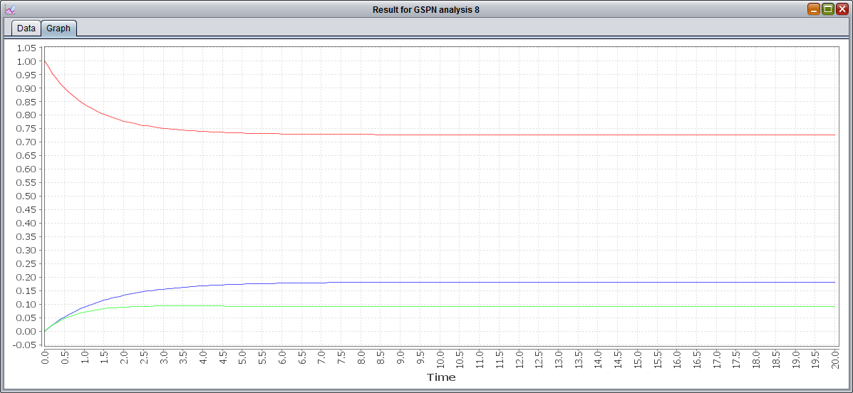
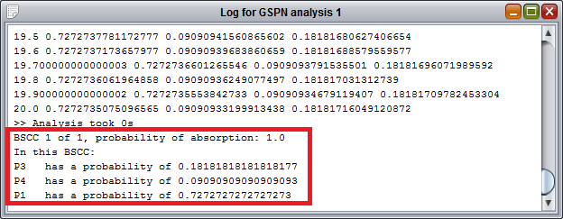
After a first transitory phase, we can see that the model reaches a steady state pretty soon. Clearly the probabilities for P3 and P4 are lower, since the execution flow of the model is split between the two after P2, with the probability of being in P3 higher since the rate of its transition is lower than P4's transition. Also we notice that P2 is not listed, being a vanishing state. If you are interested in knowing the exact value of the steady-state probabilities for these three tangible states, you can rerun the analysis with Compute steady state checked and then open the log: the result should be 0.73 for P1, 0.18 for P3 and 0.09 for P4, as you can see from this screenshot of the log:

MRP steady-state analysis

The class of Markov Regenerative Processes (MRPs) is one of the most generic and broader classes of processes underlying a PN. Due to this generality, MRP cover more cases than other simpler abstractions, but they're also usually harder to analyse.

While MRP transient analysis is covered by "Regenerative transient analysis" feature in Oris, steady-state computation can be efficiently achieved through the "Regenerative steady state analysis". This analysis, however, has the limitation of being usable only for those MRPs whose embedded DTMC in the regenerative states is ergodic, i.e. irreducible, aperiodic and positive recurrent. So, for example, the "Transmission with Timeout" net wouldn't be analysable with this method as the underlying process presents absorbing states and absorbing states are always reducible.

For this part of the tutorial, we'll then use the "Fischer's protocol" Petri Net. Once loaded into Oris, let's click on the button in order to configure the new steady-state analysis. For this analysis only a few parameters are available for configuration: it can be chose whether or not to include extended regenerations or to use the verbose logging mode and stop conditions and rewards can be specified. For this example let's say we want to evaluate the probability at steady-state for a generic process to be either waiting to enter the critical section (a.k.a. latency) or inside the critical section itself. Being the Fischer's protocol simmetric, any of the three processes can be chosen, so it's correct to focus the analysis, for example, on the first process, thus leading to the following rewards:

"ready1+writing+waiting1; cs1"

It is worth noticing that the place reading1 is not included as it is a vanishing state, providing no additional probability to the reward. Once the analysis is complete, we can open the result panel to see that the steady-state probability of being in the critical section cs1 is 0.075, while the probability of being waiting to enter in it is 0.131. If the analysis is rerun including idle1 in the rewards, it can be seen how the remaining probability is concentrated in idle1 (0.751 circa), meaning that most of the time a process is in idle mode, i.e. not needing to enter the critical section.

This PN representing the Fischer's protocol is very useful as a benchmark since many different analysis can be achieved using the Oris regenerative steady-state analysis. A couple of examples can be to compute the occupation of the critical section by any process (using "cs1+cs2+cs3" as reward) or to evaluate how the latency of a single process ("ready1+writing+waiting1") varies when the characterising parameters of the protocol, such as waiting or writing time, are changed.

Analysis under enabling restriction

Enabling restriction is the condition when, for a certain state of a PN, at most one GEN transition is enabled. If for every state of a given PN the enabling restriction is valid, the PN is then said to be under enabling restriction.

Analysis under enabling restriction is a different method to perform regenerative transient analysis, similar to the method based on stochastic state classes. The advantage is that, when analysis with stochastic state classes requires the condition of bounded regeneration to be met in order to perform it, analysis under enabling restriction requires a different condition. If we encounter a PN where bounded regeneration is not valid but enabling restriction is, it would still be analisable thanks to this new analysis.

An example PN can be "Software Rejuvenation 2", from the examples section: in this model, the bounded regeneration is not valid (transition tClock stays enabled while the cycle of EXP transitions tFProb-tDown-tUp can happen infinite times) but the enabling restriction is (trivially demonstrated, since only one GEN is present in the entire model).

In order to start a new analysis we can click on the button. For this analysis, parameters are as usual, except the allowed error which, in this case, represents the error allowed during the numerical evaluation of the embedded CTMC transient probabilities through uniformization, and not the final error on the MRP transiuent probabilities.

For the sake of this example, let's choose a time limit of 400 and a discretization step of 10. The following picture shows the graphical results of this analysis:

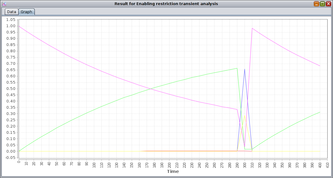
From the graphical results we can see how transient probability curves vary smoothly until the instant t=300, where many spikes are present: this is due the firing of the only GEN transition present, tClock, which is set as a DET transition with delay 300.